The standard hedge fund (HF) fee structure consists of a fixed component, the management fee, plus a performance-dependent supplement, the performance fee, that kicks-in once the HF’s annual performance exceeds a threshold value (or ‘hurdle’) for the annual return. In years like 2015, HF performance became categorically so poor that the ratio of the fee to the net returns to investors (the ‘fee load’) grew as high as 1/3, causing many investors to withdraw. The fixed management fee precludes the HF manager from sharing in the pain his investors experience during these periods. It was established because none expected those periods would appear as often as we have seen. As a HF’s returns increase from these dismal levels, the fee structure fails to reward its manager for this increase until he surpasses the hurdle. More importantly, it fails to reward the manager for performing exceptionally relative to the field of all the other managers who are his competitive peers. Whether this entire universe of HFs is facing tailwinds or headwinds in any particular year, what investors want is for their manager to still outperform to the extent currently possible. Only a relative performance fee – one that rewards the manager for superior performance relative to the field of her competitors, can provide that incentive.
I had a very detailed draft of a paper constructed on this and was ready to do the quantitative analysis to bring firm market numbers into the conceptual framework when I was suddenly separated from the computer that I had done all the work on. I dropped the whole idea, but finally decided that I can still put it out here in a very rough fashion (which seems better than just letting it die). There still is some chance I can recover a copy of my draft, and if I do, I’ll put that out as-well.
So, back to the discussion: Consider the fee level plotted as-usual on a vertical axis against the gross HF performance on the horizontal axis. At the very low end of performance, investors have some maximum fee load above which they find paying the manager intolerable. Say for example that this fee load is 1/4 (when fees become 25% of the investor’s ROI, he balks). This fee-intolerance threshold appears as a line extending upward from the origin of the plot with slope 1/4. If the manager’s performance falls down into this range where the fee has this slope, and he cannot maintain his business operations at these low levels of fee-intake, the investor may have a supplemental agreement to supply him a ‘draw fee’ to keep him going, or else he can just pull-out. The draw is basically a loan that the manager repays in later years by taking it out of the performance premium component of his annual fee.
At the high end (above the hurdle annual return of ~8%), investors are generally still happy to also pay the manager a performance fee of 10-20% of the hurdle-excess return (say this fee premium is 10%). The fee structure so far consists of a line rising from the origin with slope 1/4 until it reaches a level where it traditionally levels-off at the management fee (let this be 1%), and remains constant at that level until the gross HF return reaches the 8% hurdle, at which point it rises again with slope 0.1 due to the performance fee. This entire fee structure mirrors the traditional one except for its decay to zero as the gross return falls below 4% and declines to zero from there. So far, all these fee elements are fixed – there is no ‘relative’ element yet.
But now consider the intermediate range between 4% and the hurdle. More importantly, picture a cross-sectional distribution of the contemporaneous YTD returns of the entire field of peer HFs plotted here against the same returns axis as the fee plot. Besides the historical record of HF index data that HFRI accumulates for its clients, it also publishes (but does not store on its site) the returns of all the individual constituent HFs in its HF indices. Client firms that store this data may accumulate useful histories of these cross-sectional returns distributions (after doing a bit of appropriate compensation for the well-known biases in these data).
These distributions contain the very information on this class of HFs that is used in almost all other product markets to force the determination of their prices; namely their competitive quality relative to all their competitors’ offerings. If we divide this distribution (histogram actually) into deciles, then all the managers whose returns lie in the leftmost decile are among the lowest-performing 10% group, the ones in the rightmost decile are in the highest-performing 10%, and so-on. Starting from the left tail of this distribution, its cumulative distribution function traces a fee curve that rewards a manager with an additional unit increase in his fee each time his performance surpasses another 10% of his peers. This certainly seems a more sensible and rationally-tuned fee profile than simply drawing a straight line from the minimum value of the fee in the left tail (at, or now perhaps slightly below, 1%) up to the maximum value of the fee in the right tail (which has to be chosen).
Several advantages of allowing such a flexible fee element can be listed: (1) It allows investors to see clearly how well their manager is performing for them versus his competitors. This is not only true at year-end but also month-by-month each time the HFRI returns post and the YTD cross-sectional HF returns distribution can be updated. In essence, investors get to watch how well their “runner” (their HF manager) is placing in his race against like-managers throughout the year. (2) In years when the entire field of HFs is challenged and the distribution bunches up with a tight standard deviation down in the low-returns range, this fee still gives your manager an incentive to fight for as much performance as he can muster. But in the traditional fee, if a manager finds himself with a YTD return of 4% by Q3, and must make over 4% in Q4 to reap a performance fee, it may make more sense for him to concentrate his best-efforts elsewhere. (3) Perhaps most-importantly, it restores price-transparency to an industry in which price-opacity has been imposed by law. The laws preventing public disclosure of HF returns and fees purportedly protect unsophisticated (naive) investors, but in-truth the only people they protect are mediocre HF managers, particularly those who are good asset-gathers (marketers and client-relators). These are managers that have a good-enough story to retain investors while continuing to deliver returns below the performance hurdle, and (for awhile) make their living solely off of the management fee. Using HFRI data in this cross-sectional returns methodology will allow institutional investors restore a good deal of price-of-performance transparency (at least to themselves) under the current fee disclosure statutes. Since price and performance transparency are what drive efficiency in any market, this can only be a long-term positive for the robustness and repute of the HF industry as a whole (by weeding-out those asset gatherers over time).
I hope this post has described enough of the essence of my idea on relative performance fees (and clearly enough) to convey not only its rough conceptual framework, but also the merits for it. There are details with issues that need to be highlighted and resolved, and I hope to recoup my prior draft so I can put all that out. The draft describes another way besides the cumulative distribution function to construct the relative performance fee curve based on the returns distribution – one that may reward managers based upon their competitiveness with an even finer-tuning.
The essence of the idea can be summarized figuratively by again considering runners competing in a (marathon) race in-analogy to HF managers competing against each other in their annual performance battles: Sometimes the race course may be particularly challenging to all racers due to features like altitude and hills – just as in some years markets are more difficult for everyone. In others they may be more favorable than normal (a cool, flat sea-level race track, or a liquid market with tailwinds). In either case, a fixed absolute outperformance metric (e.g. the record marathon time, or a fixed HF performance hurdle) will always remain meaningful and highly-regarded. However, in the most challenging races the competitors most deserving of recognition and reward are not the ones who beat these fixed performance thresholds because in those instances that is usually impossible: they are the ‘top-dogs’ who solidly beat their pack of competitors. In virtually every competitive setting, people will agree that such recognition and reward is warranted. So far in HF management, it has not been.
Conversely, in friendlier race conditions, the competitors who surpass the fixed performance metric may not all be highly exceptional ones (although this is not a problem in finance, since investors are still happy to pay performance fee premia when returns are this high). Although I need an archived history of HFRI cross-sectional data to carry-out the back proof-testing of these relative fee structures for a publication, note that such a history is unnecessary to implement them. As long as an institution has an HFRI data feed, the requisite real-time HF performance data can be stored and these YTD performance distributions constructed contemporaneously, starting from January. The relative fee structures can then be constructed from them as-indicated.
I welcome any inquiries on these fee ideas: IM me on LinkedIn, or email me at slchristie6760@gmail.com. Thanks, Steve Christie.
